Tile and De-Trend

Tile the Inverse Problem and detrend the data

# sphinx_gallery_thumbnail_number = 2
import gdc19

import numpy as np
from discretize import TreeMesh
from discretize.utils import meshutils
import omfvista
import matplotlib.pyplot as plt
from matplotlib.patches import Rectangle
from SimPEG.Utils import mkvc, modelutils, PlotUtils, plot2Ddata
import pyvista

Load the Data

Load the mesh and data from the previous example

grav_data = pyvista.read(gdc19.get_gravity_path('grav_obs.vtk'))
xyz = grav_data.points
survey = pyvista.PolyData(xyz)

mesh = TreeMesh.readUBC(gdc19.get_gravity_path('mesh.msh'))
actv = mesh.readModelUBC(gdc19.get_gravity_path('actv.mod'))

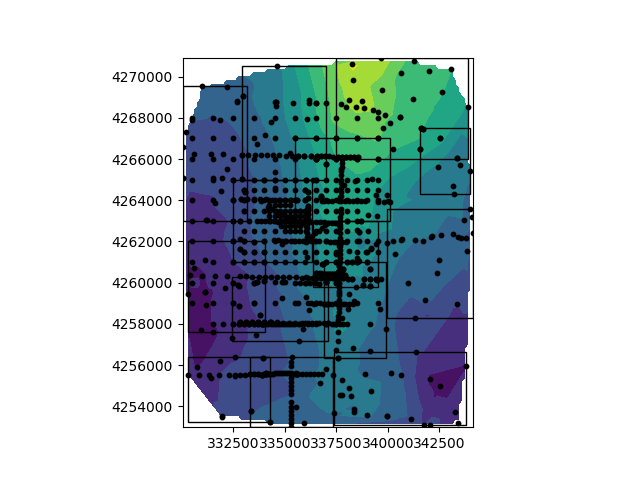
Tile the Problem

rxLoc = xyz
tiles, binCount, labels = modelutils.tileSurveyPoints(rxLoc, 14)

# Grab the smallest bin and generate a temporary mesh
indMin = np.argmin(binCount)

X1, Y1 = tiles[0][:, 0], tiles[0][:, 1]
X2, Y2 = tiles[1][:, 0], tiles[1][:, 1]


nTiles = X1.shape[0]
fig, ax1 = plt.figure(), plt.subplot()
PlotUtils.plot2Ddata(rxLoc, grav_data.point_arrays['gCBGA'], ax=ax1)
# ax1.scatter(rxLoc[:, 0], rxLoc[:, 1], 10, c='r')
for ii in range(X1.shape[0]):

    ind_t = np.all([rxLoc[:, 0] >= X1[ii], rxLoc[:, 0] <= X2[ii],
                rxLoc[:, 1] >= Y1[ii], rxLoc[:, 1] <= Y2[ii]],
               axis=0
        )
    ax1.scatter(rxLoc[ind_t, 0], rxLoc[ind_t, 1], 10, c='k')
    ax1.add_patch(Rectangle((X1[ii], Y1[ii]),
                            X2[ii]-X1[ii],
                            Y2[ii]-Y1[ii],
                            facecolor='none', edgecolor='k'))


ax1.set_xlim([X1.min()-20, X2.max()+20])
ax1.set_ylim([Y1.min()-20, Y2.max()+20])
ax1.set_aspect('equal')
plt.show()

Out:

/Users/bane/Documents/school/Masters/csm-wteam-github/GeothermalDesignChallenge/project/gravity-inversion/02-tile-detrend.py:68: UserWarning: Matplotlib is currently using agg, which is a non-GUI backend, so cannot show the figure.
  plt.show()

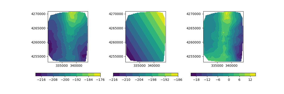
Detrend the Data

Remove regional trends from the gravity observations.

# Data[X,Y,Z,Mag]
nD = rxLoc.shape[0]
dobs = grav_data.point_arrays['gCBGA']
A = np.c_[np.ones(nD), rxLoc[:,:2]]

# Compute least-squares solution for poly parameters
poly = np.linalg.solve(np.dot(A.T,A), np.dot(A.T,dobs))

# Generate the first-order trend on each points
d = np.dot(A,poly)

dataDetrend =  dobs - d

# Plot it out
fig = plt.figure(figsize=(12,4))
ax1 = plt.subplot(1,3,1)
im = plot2Ddata(rxLoc, dobs, ax=ax1)
plt.colorbar(im[0], orientation='horizontal')

ax2 = plt.subplot(1,3,2)
im = plot2Ddata(rxLoc, d, ax=ax2)
plt.colorbar(im[0], orientation='horizontal')

ax3 = plt.subplot(1,3,3)
im = plot2Ddata(rxLoc, dataDetrend, ax=ax3)
plt.colorbar(im[0], orientation='horizontal')